Building a Linear Regression Model with Gradient Descent from Scratch

The inspiration for this project came from Andrew Ng’s “Machine Learning” course on Coursera.org. The projects for that course used Octave math coding language, which has many similar functions to Python’s Numpy library. With that in mind, I decided to practice what I learned by building a Logistic Regression model from scratch in Python. I chose a simple gradient descent method for training the model weights and then tested my code with the famous “Iris” dataset that comes packaged with Python’s Scikit Learn library.

Skills Demonstrated

• Python Libraries: Numpy, Seaborn, Pandas
• Logistic Regression coded with vectorized array functions
• Gradient Descent, also with vectorized array functions

The Data

The first use of the Iris dataset is credited to Sir R.A. Fisher, and the data has frequently been used in demonstrating pattern recognition and classification in machine learning. For this project, I elected to use the version of the data that comes packaged with the Scikit Learn Python library. The target variable is the iris species, with three possible values. It is a small dataset with 150 rows and four features. The observations are divided evenly into 50 rows of each species, and there are no missing values.

Data Features:

• Sepal Length (cm)
• Sepal Width (cm)
• Petal Length (cm)
• Petal Width (cm)

Target Variable: Species

• setosa
• versicolor
• virginica

Visualizing the Data

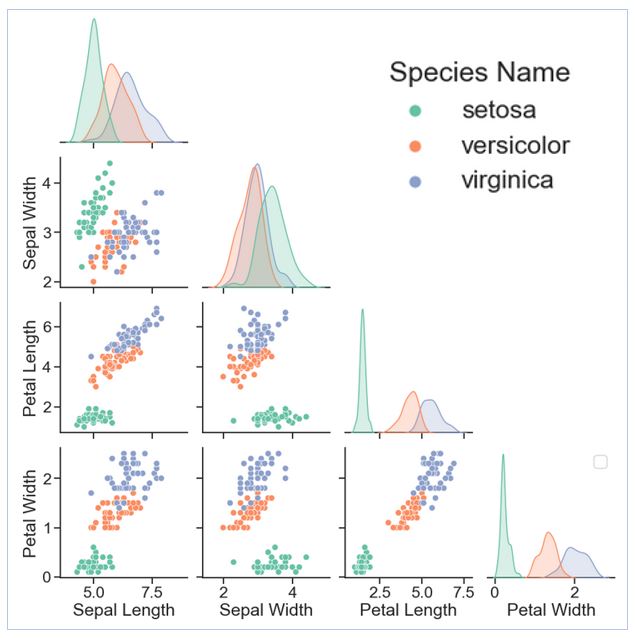
The scatter plots below, color-coded by iris species, show the relationships among the variables. In particular, petal length and petal width appear to have a positive linear relationship across the three species. We also see that setosa (green dots) has distinctly different petal and sepal measurements from the other two species. So, at a glance, one would expect the model to perform consistently well on setosa. On the other hand, the measurements for versicolor and virginica (coral and blue dots) overlap in the plots. So, one might expect the model to be somewhat less accurate in classifying these two species.

Figure 1: Pair plots comparing the relationships among data features

Python Code for Loading the Data and Creating the Pair Plots

# Tables, arrays, and linear algebra
import numpy as np
import pandas as pd

# Datasets library
from sklearn import datasets

# Visualize the data
import seaborn as sns
sns.set_theme(style="ticks")
import matplotlib.pyplot as plt

# Load the data
iris = datasets.load_iris()

# Create a dataframe and set column labels
iris_df = pd.DataFrame(iris.data)
iris_df.columns=['Sepal Length',
  'Sepal Width',
  'Petal Length',
  'Petal Width']
iris_df['Species Code'] = iris.target

# Map iris species names to a new column
spec_names = iris.target_names
iris_df['Species Name'] = iris_df['Species Code'].apply(lambda x: spec_names[x])

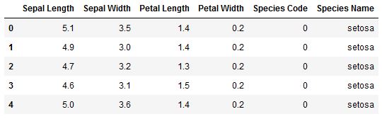
Figure 2: The first five rows of the Iris dataframe

# Context adjusts the font size and proportions of the graphics
sns.set_context("talk", font_scale=1.4)

# Create the plot
# Species Code is dropped since it is an integer code for the species name
plot = sns.pairplot(iris_df.drop('Species Code', axis=1), 
             hue="Species Name", 
             palette="Set2", 
             height=3.2,
            corner=True)

plt.show()

The Model: Logistic Regression with Gradient Descent

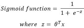
Logistic regression uses the sigmoid function to model values between 0 and 1, which makes it useful for modeling True/False classifications. In this model form, the inputs are an array of X values and a corresponding array of trained weights (also known as coefficients). Equation 1 illustrates the general form of the model in mathematical symbols.

When choosing among multiple classes of the target variable, y, a different set of model weights is trained for each class. After training, probability predictions are made using the weights for all classes and each row of X data. Final predictions are determined by finding the maximum class probability prediction for each row.    

z can also be written in its expanded form, using Numpy indexing from zero:

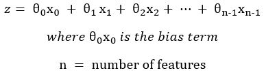
The variables in the above equation are:

• X = the inputs values (measurements of parts of the iris, in this case)
• y = the classification of each iris’s species
• θ = theta, representing an array of weights for each classification

Calculation Notes:

The leftmost (subscripts zero) term is the bias term, and the value of x0 in this term is actually “1.” Written in its long form, term-by-term, the equation for z could be written without x0. However, adding a column of ones to the 2D array/matrix X makes the implementation nicer in Numpy. Note that some texts begin indexing at 1. However, I chose to label the equations indexed from 0 to be consistent with the Python code later in this article.

I kept the superscript T (meaning transpose) in the equation for purposes of textbook notation. However, the intention is for each individual x value to be multiplied by its corresponding θ coefficient for all rows of data. During Numpy implementation, I found it simpler to reverse the order of the terms and instead do matrix multiplication of X times θ (not transposed).

Also, while θ is referred to here as model “weights,” it functions similarly to coefficients used in algebra. I have seen notation differ across texts, but the general idea is that X represents multiple x values of the data collected. The θ values are being optimized to produce the smallest amount of error when X values are input into the trained model.

The functions I coded for the Logistic Regression model are:

1. Sigmoid function
2. Cost function (a derivative of the sigmoid function)
3. Gradient computation function (derivative of the cost)
4. Gradient descent function to solve for theta
5. Model training function for a binary y array
6. Model training function for y with multiple classes
7. Predict probabilities for all classes

Additional function used: Numpy’s argmax function to find the column index for class that has the highest probability for each row

Python Code for the Training and Testing the Model

# Sigmoid Function
def sigmoid(z):
    return 1 / (1 + np.exp(-1 * z)) 

# COST of Logistic Regression

# Inputs:
# X (without bias term) & y
# theta = weights, as a 2D array
# lam = regularization term lambda
# Returns cost (J)

def lr_cost(theta, X, y, lam):
    
    J = 0  # Initialize cost
    m = X.shape[0] # Number of examples/rows
    X = np.hstack((np.ones((1, m)).T, X))# Add ones for the bias theta
    
    # Check for case where a 1D array is passed in
    if len(theta.shape) == 1: 
        theta = theta.reshape((len(theta), 1))

    # First row of theta is for the bias term
    theta_reg = theta.copy()
    theta_reg[0] = 0  # Set bias term to zero
    
    tiny = .00000001 # a very small value
        
    # Regularization term
    reg_term = lam/(2 * m) * (theta_reg.T @ theta_reg)
    
    # Cost
    log_loss = 1/m * np.sum(
        (-1 * y * np.log(sigmoid(X @ theta) + tiny) 
         - (1 - y) * np.log(1 - sigmoid(X @ theta)+ tiny))) 
    
    J = log_loss + reg_term

    return J 

# GRADIENT of Logistic Regression

# Inputs:
# X (without bias term) & y
# theta = weights, as a 2D array
# lam = regularization term lambda
# Returns gradient(grad)
def lr_gradient(theta, X, y, lam):
    
    # Check for cases where a 1D array is passed in
    if len(theta.shape) == 1: 
        theta = theta.reshape((len(theta), 1)).copy()
    
    if len(y.shape) == 1: 
        y = y.reshape((len(y), 1)).copy()
        
    m = X.shape[0] # Number of examples/rows
    grad = np.zeros(theta.shape)    # Initialize gradient   
    X = np.hstack((np.ones((1, m)).T, X))# Add ones for the bias theta
    
    # First row of theta is for the bias term
    theta_reg = theta.copy()
    theta_reg[0] = 0  # Set bias term to zero
    theta_reg = lam/m * theta_reg  # Gradient Regularization term 
    
    # keepdims option tells numpy sum not to flatten the axis of the result
    grad = np.sum((1/m * (sigmoid(X @ theta) - y) * X).T 
                  , axis=1
                  , keepdims=True) + theta_reg
    
    #print(grad)
    
    return grad

# GRADIENT DESCENT
def gradient_desc(theta, X, y, lam, num_iters, alpha):
     
    m = X.shape[0] # Number of examples/rows

    # Check for 1D arrays (from using optimizers that flatten arrays)
    if len(y.shape) == 1: 
        y = y.reshape((len(y), 1)).copy()
    
    for i in range(num_iters):
        grad = lr_gradient(theta, X, y, lam)
        J = lr_cost(theta, X, y, lam)
        
        if i%100 == 0: print("Iteration: ", i, "Cost: ", J)
            
        # update theta
        theta = theta - alpha * grad
       
    return theta

# TRAIN with Binary y

# Solve for Theta with simple binary y values
# lam = lamda in regularization terms
def lr_train(X, y, lam, num_iters, alpha):
    
    theta_size = X.shape[1] + 1
    init_theta = np.ones((theta_size, 1)) + .05

    theta = gradient_desc(init_theta, X, y, lam, num_iters, alpha)
    
    return theta

# TRAIN with Multiple Class y

# Solves for Theta with multiple classes
# Returns
# - all_thetas: 2D array of thetas for ALL classes
# - class_array: array of class names, indexed same order as thetas
def lr_train_multi_class(X, y, lam=1, num_iters=1000, alpha=0.1):

    (m, n) = X.shape
    classes = np.unique(y)    
    
    # Initialize 2D array of thetas
    all_thetas = np.ones((n + 1, classes.shape[0]))
    
    i = 0
    for c in classes:
        
        print("Class: ", c)
        yc = np.array([1 if y == c else 0 for y in y])
    
        # Train the classifier on each class
        result = lr_train(X, yc, lam, num_iters, alpha)
        
        # Append predicted results as a new (row/col?) 
        all_thetas[0:, i] = result.flatten()

        i += 1

    return all_thetas, classes

# PREDICT
# For multi class, each class's theta is a column vector
def lr_predict_prob_all(theta, X):
    
    (m, n) = X.shape
    X_ones_col = np.ones((1,m)).T
    
    # Check for case where a 1D array is passed in
    if len(theta.shape) == 1: 
        theta = theta.reshape((len(theta), 1))
    
    # Add a column of ones for the bias term in theta
    X = np.hstack((X_ones_col, X))
    
    # Predict all probabilities
    return sigmoid(X @ theta)

Results

To test my code, I trained three models, plus one extra with Scikit Learn’s logistic regression classifier. To keep training results consistent, I used the same lambda, alpha, and number of iterations for all three gradient descent models. I also split the data into 67% training rows and the remaining 33% as test rows. If the dataset had more observations, I would have also liked to split some rows off into a validation set. However, given that the entire dataset had only 150 observations, it seemed impractical to split it further.

Inputs for all three gradient descent models:

• lambda = 0.9,
• number of iterations = 1500,
• alpha = 0.01

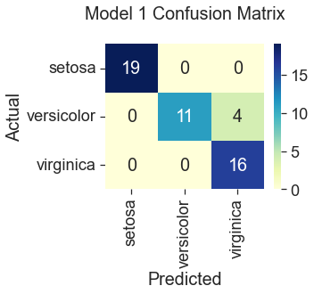
Model 1: Gradient Descent with All Features

92% Accuracy

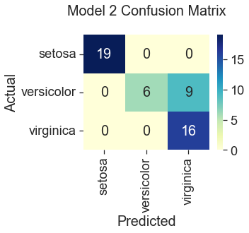
Model 2: Gradient Descent with Only ‘Sepal Width’ and ‘Petal Width’

82% Accuracy

Model 3: Scikit Learn’s Logistic Regression with All Features, Default Parameters

100% Accuracy

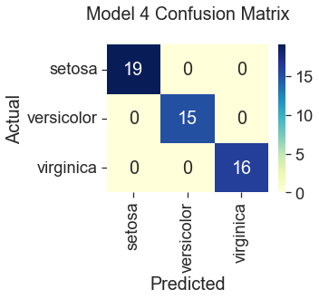
Model 4: Gradient Descent with Polynomial Terms, All Features

100% Accuracy

Conclusion

All three gradient descent models predicted correctly for the species setosa. This result is consistent with what we saw in the plots during the data visualization step, where setosa was represented by clusters of green dots that had noticeably different measurements from the other two species. The least accurate model (82%) was gradient descent trained with only two features, “Sepal Width” and “Petal Width.” Compare this to Scikit Learn’s logistic regression model, which performed the best at 100% accuracy using the four original features. Gradient descent also predicted the iris species with 100% accuracy when additional features were engineered by squaring the original iris measurements. However, this additional step seems unnecessary when the Scikit Learn model can produce the same accuracy using the unengineered features. So, I would select the Scikit Learn model for its ease of use.

Accuracy of the Results

Accuracy of 100% would usually be reason to suspect that something was amiss. Perhaps some variation of the target variable had been used as a feature to train the model. However, in this case, the dataset is small and very simple. Furthermore, the plots showed that at least one of the species could be neatly separated based on sepal and petal measurements, with no overlap into the measurements of other species. So, it seems more likely that the data in this case is simply very consistent. For these reasons, I concluded that the models are good, given the limited number of observations.

References

Ng, Andrew. Machine Learning. Coursera.org. www.coursera.org/learn/machine-learning

(1988). Iris [Data set]. Scikit Learn Python Library. scikit-learn.org/stable/auto_examples/datasets/plot_iris_dataset.html